




Initial analysis as of 20 August 2026
For a summary of the key findings, see our press release
→ https://prtimes.jp/main/html/rd/p/000000008.000180454.html (only Japanese)
Damage Summary (GIS format)
→ https://summaries.aqunia-floods.aqunia.com/summaries/1/en_us/
About this article
This article summarizes publicly available materials and the results of our own numerical analysis of the heavy rainfall that struck Chiba Prefecture on 13–14 August 2026.
This was a disaster that left 13 people dead and 1 missing. A full investigation of causes should properly take far more time; we publish this piece because we believe it has value in providing an initial understanding as various discussions proceed. The results here are preliminary and may change with further scrutiny. We welcome corrections if anything is wrong.
This analysis was conducted as part of Aqunia’s ongoing development of meteorological and hydrological models. We first present results based mainly on JMA MSM-GPV, Composite Radar GPV, JMA AMeDAS, and specialized weather charts.
Intended readers: journalists; disaster-management officials in national and local government; and private-sector practitioners in construction consulting, insurance, infrastructure, manufacturing, and related disaster-risk fields
Part 1 — What happened
1-1. Overall picture of the damage
The 13–14 August 2026 heavy rainfall caused an unusually severe human toll for a flood disaster: 13 dead and 1 missing (Chiba Prefecture official tally, Report No. 14, issued 16:00 on 19 August 2026). Most deaths involved people found in vehicles or on roads during flooding. Building damage was also extensive, with 1,206 buildings flooded above floor level and 1,489 flooded below floor level. Notably, 55.7% of the damage occurred outside flood hazard map inundation zones and low-lying areas (Weathernews mapping of 10,009 flooding-status survey responses) — a defining feature of this event.
A map-based overview of the damage is available at the link below.
▶ Damage Summary (GIS format): https://summaries.aqunia-floods.aqunia.com/summaries/1/en_us/
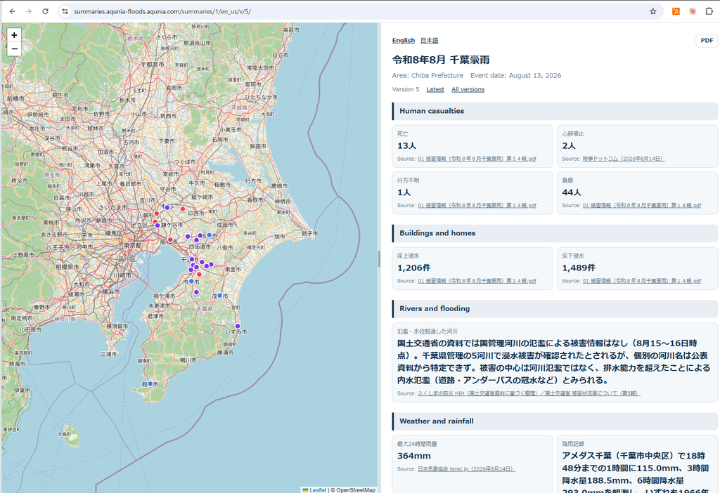
This summary was produced using Aqunia Flood’s admin “Damage Summary” feature, which combines generative AI with GIS to automatically generate damage reports from various data sources.
Note on how to read the numbers
The death toll was initially reported as 10 in the prefecture’s official count (as of 17 August), conflicting with some media reports of 13; Report No. 14 on 19 August revised the official figure to 13. Missing persons fell from 2 to 1. Cases of carbon monoxide poisoning (generator use) and cases still under review for disaster causality are also included. Media reports immediately after the disaster of “45 buildings above-floor / 39 below-floor flooding” were early tallies; the final figures are more than 20 times higher.
Infrastructure damage was also widespread. Power outages peaked at about 25,900 households (of which about 15,890 were linked to flooding of the Soga substation); roads saw full closures on 25 routes due to surface flooding, slope failures, and abandoned vehicles; and three wastewater treatment facilities stopped functioning due to flooding. Manhole overflows occurred at 8 locations, and uplift or lid damage at 6. Abandoned vehicles ultimately numbered at least 2,800. Shelters housed up to 4,126 people (Report No. 14, Appendix 4; person-based, excluding evacuated households). Stranded travelers numbered about 4,000 around Soga Station, about 6,600 at Narita Airport, and about 1,600 at Chiba Prefectural Government.
This damage distribution itself leads into the discussion of urban (pluvial) flooding later in the article. The highest above-floor flooding was in Yachiyo City (327 buildings), followed by Oamishirasato City (200) and Chiba City (179). The highest below-floor flooding was in Matsudo City (315), followed by Kamagaya City (213). None of these municipalities correspond to any of the eight rivers for which Level 4 flood danger information was issued. Details are covered in Part 4.
1-2. Timeline: rainfall and warnings
Rainfall records
On 14 August, JMA named this event the “August 2026 Chiba Heavy Rain” (Reiwa 8 August Chiba Heavy Rain). It was the first time in six years that JMA had named a meteorological phenomenon since the July 2020 heavy rain, and the first time in nine years that a regional name had been included since the July 2017 Northern Kyushu heavy rain.
Records that set all-time highs (from Choshi Local Meteorological Observatory, “Chiba Prefecture Weather Bulletin Report No. 2,” with timestamps).
1-hour precipitation
| Station | New record | Time reached | Previous No. 1 | Records since |
|---|---|---|---|---|
| Chiba (Chuo Ward) | 115.0 mm | 8/13 18:48 | 71.0 mm (1975/10/5) | 1966 |
| Sakura | 97.0 mm | 8/13 19:31 | 68.5 mm (2015/6/23) | 1976 |
| Tateyama | 94.5 mm | 8/13 21:53 | 74.5 mm (1972/9/15) | 1968 |
| Funabashi | 62.0 mm | 8/13 18:43 | 58.5 mm (2013/10/16) | 1999 |
| Abiko | 61.0 mm | 8/13 14:30 | 53.5 mm (2016/7/20) | 2010 |
By duration (Chiba)
| Duration | New record | Time reached | Previous No. 1 |
|---|---|---|---|
| 3 hours | 188.5 mm | 8/13 19:30 | 137.5 mm |
| 6 hours | 293.0 mm | 8/13 23:20 | 211.0 mm |
| 12 hours | 348.0 mm | 8/14 01:40 | 267.5 mm |
| 24 hours | 367.0 mm | 8/14 10:00 | 309.0 mm |
For 3-hour rainfall, Sakura recorded 189.5 mm (19:50), the highest in the prefecture. In both Chiba City and Sakura City, about three times the normal August monthly precipitation (115.7 mm and 109.1 mm, respectively) fell in two days.
Sequence of warnings and linear precipitation band information
| Time | Event |
|---|---|
| 8/12 16:00 | Disaster-prevention email (alerts began the previous day) |
| 8/13 05:05 | Heavy rain advisory (Level 2, 2 cities) |
| 8/13 13:52 | Heavy rain warning (Level 3) |
| 8/13 14:30 | Abiko: 61.0 mm in 1 hour (all-time high) |
| 8/13 17:05 | Heavy rain emergency warning (Level 4) |
| 8/13 17:12 | Chiba Prefecture Weather Commentary Information No. 10 |
| 8/13 17:28 | Record short-term heavy rain information No. 1 (approx. 110 mm in Kashiwa City, approx. 100 mm in Abiko City) |
| 8/13 ~17:30 | First human casualty (Kashiwa City, flooded vehicle) |
| 8/13 17:35 | Mayoral hotline begins (Kashiwa City) |
| 8/13 17:58 | Linear precipitation band occurrence No. 1 |
| 8/13 18:48 | Chiba: 115.0 mm in 1 hour (all-time high) |
| 8/13 18:58 | Linear precipitation band nowcast No. 1 |
| 8/13 19:28 | Linear precipitation band nowcast No. 2 |
| 8/13 19:30 | Heavy rain special warning (Level 5, 11 cities) |
| 8/13 19:50–8/14 00:40 | Special warning expanded stepwise → finally 19 cities and 3 towns |
| 8/13 20:30 | Joint MLIT–JMA press conference |
| 8/13 20:38 | Linear precipitation band nowcast No. 3 |
| 8/13 20:58 | Linear precipitation band occurrence No. 2 |
| 8/13 21:00 | Meteorological Observatory briefing on the special warning |
| 8/13 21:55 | Landslide special warning (Chiba City, Ichihara City) → finally 6 cities |
| 8/13 22:00 | JETT (JMA Emergency Task Team) dispatched to prefectural government |
| 8/13 22:48 | Linear precipitation band nowcast No. 4 |
| 8/13 ~23:40 | Overbanking begins on the Murata River (Daido Bridge) |
| 8/14 00:18 | Mayoral hotline ends (23 municipalities, 36 calls in total) |
| 8/14 02:08 | Linear precipitation band occurrence No. 3 |
| 8/14 02:36 / 03:33 | Tornado advisory No. 1 / No. 2 |
| 8/14 05:15 | Special warning stepped down to Level 4 |
Record short-term heavy rain information was issued a total of 25 times.
What this timeline shows
Escalation did follow the stages. Advisory (05:05) → warning (13:52) → emergency warning (17:05) → special warning (19:30): a stepwise escalation over 14 hours 25 minutes. The mayoral hotline reached 23 municipalities with 36 calls. Information flow to government was dense.
Even so, it could not get ahead of the casualties. The first human casualty was in Kashiwa City around 17:30. Record short-term heavy rain information No. 1 was issued at 17:28 (about 110 mm in one hour near Kashiwa City). The two were essentially simultaneous. Between the emergency warning (17:05) and the special warning (19:30)—2 hours 25 minutes—people had already died.
The effective lead time of linear precipitation band information varied greatly by occurrence.
| Occurrence notice | Target area | Preceding nowcast |
|---|---|---|
| No. 1 17:58 | Northwest, south | None (first nowcast was 18:58 = 60 minutes after occurrence) |
| No. 2 20:58 | Northwest, northeast, south | 18:58 / 19:28 / 20:38 (by area; 20 minutes–2 hours) |
| No. 3 8/14 02:08 | Northwest, northeast | 22:48 (but 20 minutes beyond the 3-hour validity window) |
For No. 1, the nowcast did not arrive in time. That said, this is limited to the linear precipitation band product family; the heavy rain emergency warning (17:05) and record short-term heavy rain information No. 1 (17:28) had already been issued.
For No. 2, a nowcast was issued 20 minutes ahead. Short as that is, the system functioned as designed.
For No. 3, a preceding nowcast existed, but the gap was 3 hours 20 minutes. Because nowcast validity is defined as 3 hours, this interval exceeds the system’s design assumption. Rather than treating the 22:48 nowcast as having captured the 02:08 occurrence, it may be more appropriate to treat it as a re-issuance for a separate event, or for a continuing phenomenon.
Note that operational use of linear precipitation band nowcasts began on 28 May 2026; this case came only about two and a half months later. Hit rates are expected around 50%, which already looks like a substantial improvement relative to earlier half-day-ahead forecasts. Given how new the product is, judging its effectiveness from a single case would be premature; it is better to see this event as the first major test of the new system. We see both a degree of usefulness and issues that still need to be worked through.
We believe the role of the special warning deserves credit. At the 19:30 issuance, Chiba had already recorded 188.5 mm in 3 hours (reached at 19:30), so the special warning partly addressed “what was already happening” rather than only “what was about to happen.” Even so, a second (20:58) and third (02:08) linear precipitation band followed. As a signal to prepare for the second and third bands, it functioned quickly and effectively. This was the first Level 5 heavy rain special warning since the May 2026 revision of disaster meteorological information operations. Personally, we believe that revision made the Level 5 design easier to understand.
1-3. Decomposing risk
Disaster risk is generally decomposed as
Risk = Hazard × Vulnerability × Exposure
Hazard denotes the magnitude of the natural phenomenon (e.g., heavy rain and flooding, strong winds). Even with an extreme natural disaster, resilient infrastructure may limit damage; conversely, insufficient infrastructure—especially in developing countries—can amplify it. That dimension is “vulnerability.”
And even if infrastructure is fragile and an extreme disaster occurs, if no one lives there and no assets are present, it is not fundamentally a risk to people. The degree to which people and assets are present is “exposure.”
Applied to this case, three major drivers of the damage can be framed as follows.
- Hazard: Rain that far exceeded previous all-time highs (Chiba’s 1-hour rainfall was 1.6× the old record)
- Vulnerability: Warnings that could not get ahead of casualties, and urban drainage capacity not designed for 115 mm in one hour
- Exposure: 55.7% of damage occurred outside flood hazard map inundation zones and low-lying areas (Weathernews mapping of 10,009 flooding-status survey responses)
This article focuses mainly on hazard (Parts 2 and 3) and the forecast-related aspects of vulnerability (Parts 3 and 4). Exposure issues are touched on in Part 4.
Part 2 — Mechanism: why this rain occurred
2-0. It cannot be reduced to a single phrase
Media coverage circulated keywords such as “monsoon gyre” and “back-building and side-building linear precipitation bands.” Individual points each have a basis, but listing keywords is not an explanation.
In the end, rain falls through the following steps.
- Water vapor is present (supply)
- It is lifted (instability sets how readily it rises; forcing pulls the trigger)
- It becomes cloud and rain
- When that persists in the same place, it becomes damaging heavy rain (quasi-stationarity)
Viewed across these four layers, this event can be explained qualitatively in large part. Below we check each with data.
JMA (Choshi Local Meteorological Observatory) describes the event officially as follows.
Over the Kanto–Koshin region on the 13th–14th, unusually strong cold air for the season flowed aloft, and warm, moist air streamed in around the rim of a high over the east of the Kurils, making the atmosphere extremely unstable. In Chiba Prefecture, from the early afternoon of the 13th onward, cumulonimbus clouds organized over the northwest, south, and northeast, linear precipitation bands formed (abbreviated), and record heavy rain occurred in many places.
The official account cites two elements: “cold air aloft” and “warm moist inflow around the rim of a high.” Cold-air outflows and convergence zones are not mentioned in the written statement (at the 8/13 20:30 press conference, Forecast Division Director Hosomi did state orally that “clouds stalled where they collided with winds from the north”). The cold-pool and opposing-flow discussion below does not negate the official explanation; it adds our hypothesis on top of it.
The term “monsoon gyre” does not appear in JMA official materials, and its definition seems somewhat fluid, so we avoid asserting it here.
2-1. Moisture supply: “moisture left by Typhoon 15” is not entirely wrong—but it is not precise
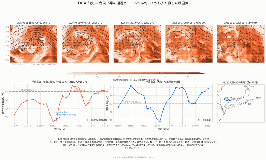
Typhoon 15 made landfall in Kanto on the night of 11 August and became a tropical depression on the 12th. The idea that “warm moisture left by that typhoon caused the heavy rain” is intuitively appealing, but the data suggest some caution is needed.
Tracking 850 hPa equivalent potential temperature (θe; a combined measure of warmth and moisture) and precipitable water (total column water vapor) directly over Chiba yields the following.
| Time | 850 hPa θe | Precipitable water |
|---|---|---|
| 8/11 12 UTC (typhoon passage) | 339.9 K | 61.0 mm |
| 8/12 12 UTC | 327.6 K | 40.8 mm |
| 8/13 06 UTC | 348.4 K | 60.0 mm |
| 8/13 12 UTC (during heavy rain) | 347.6 K | 60.0 mm |
It dried out substantially in between. Precipitable water fell from 61 mm to 41 mm, and θe from 340 K to 328 K. From the morning of the 13th, moisture re-entered afresh, returning to 348 K / 60 mm during the heavy rain. The air that exceeded the heavy-rain rule of thumb of 850 hPa θe = 345 K was the air that re-entered on the 13th.
So the causal chain is as follows.
Typhoon 15 did not leave moisture behind. The same high-pressure configuration that steered Typhoon 15 onto its unusual westward track continued to send easterly flow after the typhoon departed, and re-imported water vapor on the 13th.
The Tokyo Shimbun’s statement that “the high near the Kurils is also thought to have put Typhoon 15 on its unusual westward track, and that influence lingered” is consistent with this picture. There is a connection to the typhoon’s motion, but the typhoon itself did not directly deposit the moisture.
The distinction looks fine-grained, but it matters in practice. The judgment that “the typhoon has gone, so we are safe” did not hold in this case. Conditions reset after a dry-out following the typhoon’s departure.
2-2. Instability: a vertically coherent cut-off cold vortex
What was happening at ~5,000 m
The center of the low at 500 hPa (~5,700 m) moved as follows.
| Time | Low center | 500 hPa temperature over Chiba |
|---|---|---|
| 8/12 00 UTC | 34.0°N / 138.1°E | −5.9 °C |
| 8/12 12 UTC | 34.0°N / 136.3°E | −8.2 °C |
| 8/13 00 UTC | 37.0°N / 132.0°E | −7.2 °C |
| 8/13 12 UTC (during heavy rain) | 43.0°N / 128.0°E | −5.7 °C |
The low exited from the Sea of Japan toward the continent, and Kanto remained on its southeast side—ahead of the trough. The 500 hPa temperature over Chiba stayed around −6 °C, maintaining an unstable stratification of warm-moist air below and cold air aloft.
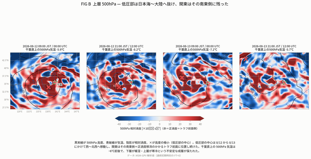
Specialized chart readouts (AUPQ35 analysis) also place the “−6 °C contour near Kanto,” in good agreement with the MSM analysis value of −5.7 °C.
Vertical structure: (a key point for understanding this event)
A common lesson in weather-forecaster training and chart reading is: “Looking only at the surface chart is not enough; grasp the three-dimensional structure by linking multiple upper-level layers.”
A classic example is westward tilt of a trough with height. In a developing baroclinic wave, the trough axis tilts westward with height. Cold air lies behind (west of) the trough, and the system draws energy from that configuration. As it matures, the axis becomes more vertical (equivalent barotropic).
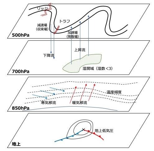
※Schematic of a typical developing cyclone (source: Reading developing cyclones)
This case was not that pattern.
FIG C is a longitude–height cross section averaged over 34.5–38.5°N. Tracking the longitude of the trough axis at each level:
| Pressure level | Trough-axis longitude |
|---|---|
| 1000 hPa | 131.1°E |
| 950 hPa | 130.8°E |
| 850 hPa | 130.6°E |
| 700 hPa | 130.0°E |
| 500 hPa | 131.8°E |
| 400 hPa | 136.3°E |
| 300 hPa | 136.5°E |
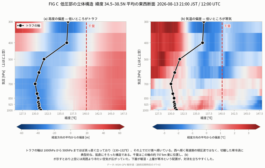
From 1000 hPa to 500 hPa, the axis stands nearly upright at 130–132°E. Eastward tilt begins only above 500 hPa. This is not westward tilt. It is the vertically aligned structure typical of a cut-off cold vortex.
And FIG C(b) (temperature-anomaly cross section) shows cold air spreading in the mid-to-upper troposphere east of the trough axis at 132–140°E. The axis itself was distant, but a cold tongue reached over Chiba. That completes the warm-moist below / cold aloft configuration.
Instability and moisture acted in sequence
FIG D shows the time evolution of the vertical structure over Chiba (35.60°N, 140.11°E). The internal order of this case is clear here.
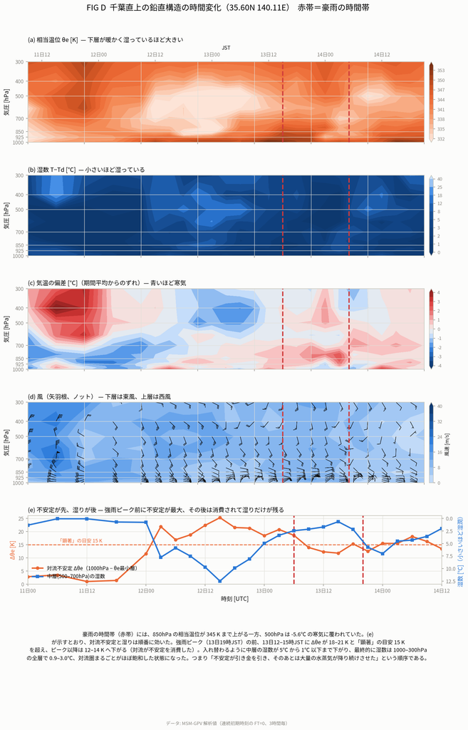
- Convective instability Δθe (difference between 1000 hPa and the θe-minimum layer) reached 18–21 K—exceeding the “notable” threshold of 15 K—at 12–15 JST on the 13th, before the heavy-rain peak (19 JST on the 13th). After the peak it fell to 12–14 K (convection consuming the instability).
- In exchange, mid-level (500–700 hPa) dewpoint depression fell from 5 °C to below 1 °C. Ultimately, dewpoint depression was 0.9–3.0 °C through the full column from 1000 to 300 hPa—a state of near saturation through almost the entire troposphere.
In short,
Instability pulled the trigger; afterward, abundant water vapor kept the rain falling.
Instability and moisture did not act simultaneously; they acted in sequence. That also matters for the predictability discussion in Part 3.
2-3. Forced ascent: cold-pool and easterly pushback
Clear signals in Chiba AMeDAS data
Looking at the Chiba AMeDAS station that recorded heavy rain is the clearest place to start.
At 18:10 JST on 13 August, the following happened at once.
- Wind direction shifted sharply from NNE → NW
- Wind speed rose to 7.9 m/s
- Temperature fell by −1.6 °C
- Pressure rose by +0.4 hPa
- 10-minute rainfall surged
Wind, temperature, pressure, and rain all bent at the same instant. This is consistent with passage of a convergence line (gust front). (FIG E, lower panel)
The cold pool in substance
The upper panels of FIG E map surface potential-temperature anomaly Δθ (difference from 15 JST) hour by hour.
Potential temperature is the temperature an air parcel would have if brought to 1000 hPa—removing elevation effects so sites can be compared fairly. Looking at its anomaly shows directly “how much cooler it became relative to before the heavy rain began.” Blue is negative = cooled air.
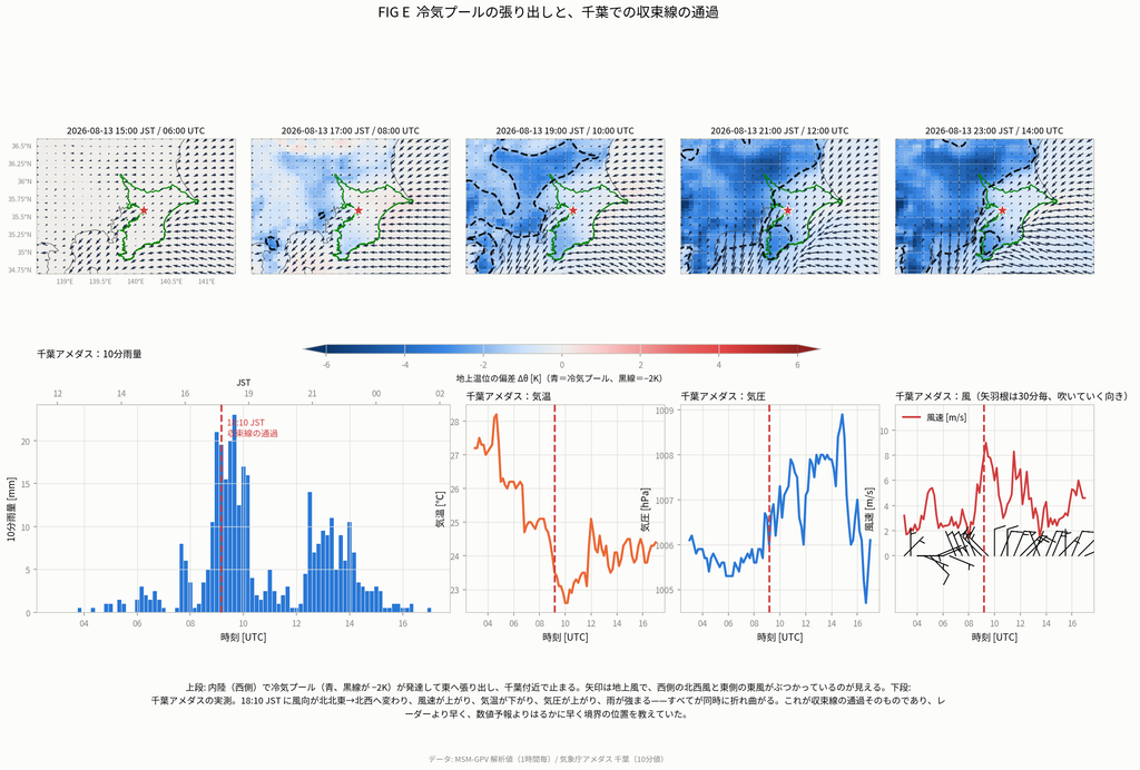
Blue spreads cleanly over western to northwestern Chiba Prefecture. Rain that began inland (Saitama to southern Gunma) from early afternoon on the 13th cooled near-surface air through evaporation, making it denser and allowing it to pool. That is the cold pool. Mean potential-temperature anomaly inside the cold pool fell to −2.6 K at 18 JST and −3.3 K at 21 JST.
This cold air spreads eastward as a density current. Its leading edge reached Chiba at 18:10.
Why did it stall there?
This is the core of the mechanism. A gust front cannot normally sit still. As long as a density difference exists, it will try to expand outward. If it did not move, an opposing force of similar magnitude must have been pushing back.
FIG 5c tests this hypothesis with three independent numbers.
| Quantity | Value | Nature |
|---|---|---|
| Theoretical cold-outflow speed C_gust (eastward) | 37 km/h | Theory (density-current formula) |
| 950 hPa easterly pushback (westward) | 28 km/h | MSM |
| Front eastward advance from AMeDAS isochrones (95 stations) | 5.1 km/h | Observed (r=0.79, 15 stations) |
| Net motion of MSM convergence-band centroid (14 hours) | 1.6 km/h | MSM |
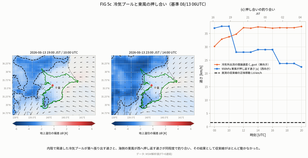
37 and 28 are of the same order and in opposition, so the boundary moved at only about 5 km/h. It is like a tug-of-war in which both sides pull hard and the rope’s center barely moves.
These numbers are calculated under assumptions, so their probability has limits. C_gust comes from the density-current formula C = √(g·Δθ/θ₀·h), assuming cold-pool depth h = 1000 m. h was not observed. Because it enters as √h, h = 500 m gives 26 km/h and 1500 m gives 45 km/h. The figure “37” has roughly ±40% width. The pushback of 28 km/h is also an MSM value, not an observation. What can safely be claimed is therefore only that they were of the same order and in opposition. “37 versus 28” should not be read as high precision.
Even so, the framing is useful. Media sometimes said a “shear line stalled,” but here we offered a hypothesis for why it stalled, in terms of a force balance, with order-of-magnitude numbers that fit. Not “it happened to stop,” but “the conditions for stopping were in place.”
However, the model placed the convergence line too far southeast
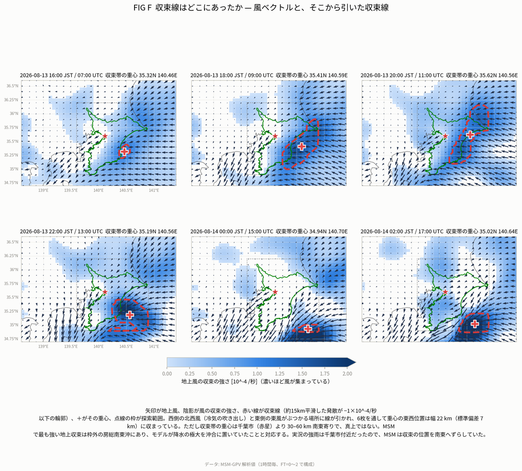
FIG F extracts a convergence line from MSM surface winds (contour of divergence smoothed over ~15 km at or below −1×10⁻⁴/s, with + marking the centroid).
| Time | Convergence-band centroid |
|---|---|
| 8/13 16:00 JST | 35.32°N / 140.46°E |
| 18:00 JST | 35.41°N / 140.59°E |
| 20:00 JST | 35.62°N / 140.56°E |
| 22:00 JST | 35.19°N / 140.56°E |
| 8/14 00:00 JST | 34.94°N / 140.70°E |
| 02:00 JST | 35.02°N / 140.64°E |
East–west position stays within a 22 km width (standard deviation 7 km). MSM itself shows that the convergence line barely moved in the east–west direction.
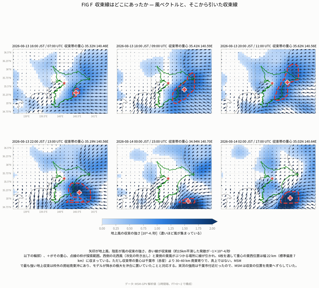
At the same time, the centroid lies 30–60 km southeast of Chiba City—not overhead. Moreover, the strongest surface convergence in MSM lay outside the search domain, over the sea southeast of the Boso Peninsula.
We regard this location bias as one cause of the underforecast of rainfall discussed later. On the 700 hPa chart as well, the strongest ascent maximum was placed just east of Chiba over the sea. Forecast rainfall distributions were similarly shifted east.
In other words, the model did reproduce the structure of the phenomenon. That a convergence line existed, and that it did not move east–west—MSM captured both. What it missed was location (30–60 km southeast) and intensity. That is an important caveat for future forecast improvement.
2-4. Quasi-stationarity: unpacking what “did not move” means
Reference figures: FIG 6b (FIG6b_escalator.png), FIG 7 (FIG7_centroid.png / FIG7_axis_profile.png / FIG7_hovmoller.png)
The clouds were moving. What did not move was “where clouds were born.”
Using 1 km radar GPV (5-minute values), we separately measured the motion of individual rain clouds and of the precipitation system as a whole over 14 hours from 8/13 06–20 UTC (15 JST to 05 JST the next day).
| Value | |
|---|---|
| Advection speed of individual rain clouds (echoes) | 22–24 km/h (toward NNW) |
| Total distance rain clouds traveled in 14 hours | 358 km |
| Net distance the rain band itself moved | 25 km = 1.8 km/h |
Rain clouds traveled 358 km in 14 hours. Yet the band moved only 25 km. What exited was continually replaced by new rain clouds forming at the rear.
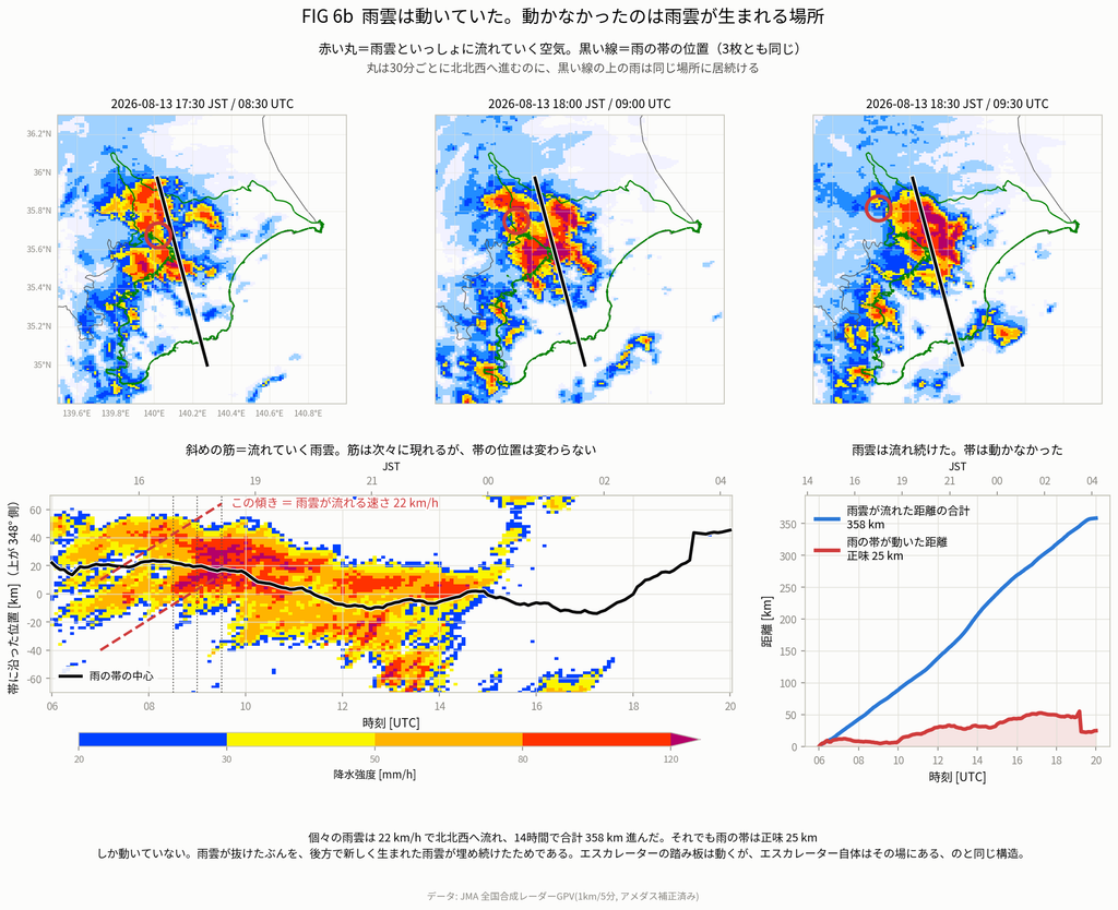
In metaphor: the escalator steps are moving, but the escalator itself stays in place. Saying “the linear precipitation band stalled” can sound as if the clouds stopped; in fact the clouds kept flowing. What was stationary was where clouds were generated.
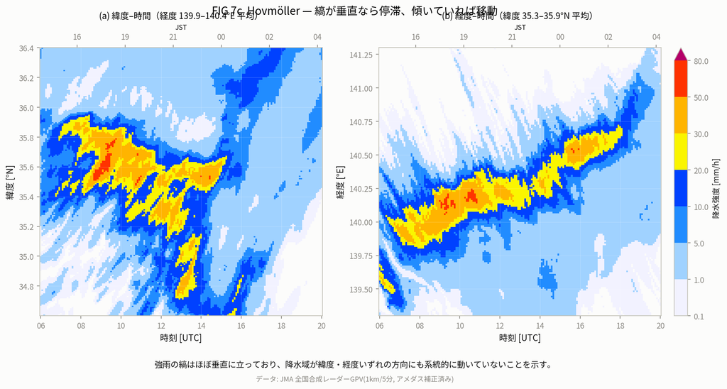
The same appears in the Hovmöller diagram (FIG 7). Individual rain clouds appear as diagonal streaks (the slant is the 22 km/h advection speed), while the line marking the band center is nearly horizontal.
Spatial structure independently corroborates this
If a precipitation system were translating, it would leave rain everywhere it passed. Accumulated rainfall would be stretched in the direction of motion, and elongation would be lost. Translation can only push the accumulation field toward isotropy.
We measured spatial gradients of accumulated rainfall in two directions relative to the precipitation axis.
| Direction | Segment | Distance | Radar | AMeDAS |
|---|---|---|---|---|
| Across-axis | Sakura → Narita | 16.1 km | 18.1 mm/km | 14.9 mm/km |
| Along-axis | Chiba → Tateyama | 71.7 km | 2.9 mm/km | 2.3 mm/km |
| Anisotropy | 6.3× | 6.5× |
Crossing the axis, rainfall falls by 18 mm per km; along the axis, by only 3 mm. Sakura and Narita are only 16 km apart, yet total rainfall split into 309 mm and 68 mm.
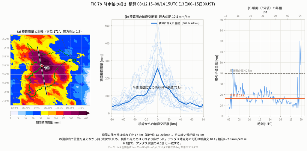
And that factor of six is produced independently by radar and AMeDAS—instrument systems that are entirely different (6.3 and 6.5). Radar estimates from microwave backscatter aloft; AMeDAS measures directly with tipping-bucket gauges on the ground. Taking a ratio cancels radar calibration coefficients in numerator and denominator. This factor of six is robust even if radar absolute values are uncertain.
The band was even narrower than often assumed
Breaking the width down further:
- Instantaneous (5-min) band width: FWHM 16.5 km (interquartile 13–20 km; n = 169 times)
- Accumulated (48-hour) footprint width: FWHM 40 km
So the accurate picture is not “a 20–30 km-wide band that did not move,” but
a ~16 km-wide band that wandered within a ~40 km-wide corridor while raining for 8 hours
Hazard maps are drawn at river-basin scale, but the precipitation itself had structure finer than a basin.
It “did not move,” yet seemed to spread south—because the direction of motion was different
Looking at how damage spread, the rain clearly appears to have moved. Peak times of 1-hour rainfall line up as
Abiko 14:30 → Funabashi 18:43 → Chiba 18:48 → Sakura 19:31 → Tateyama 21:53
From Abiko to Tateyama is about 100 km over 7.5 hours, or roughly 13 km/h on average. That seems to contradict the earlier “1.8 km/h,” but it does not. Only the direction of motion differs.
The precipitation band was a nearly north–south elongated strip. Across the band (east–west) it barely moved; along the band (north–south) it slowly slid south over half a day. Imagine a north–south string that barely shifts sideways, but slowly slides south along its own orientation.
Because it did not move sideways, the same places were rained on for hours, producing the phenomenon that Sakura and Narita—only 16 km apart—differed by more than a factor of three in rainfall. Had it moved east–west at 13 km/h, rain would have been smeared over a ~90 km width in 7 hours, and such a contrast would not arise.
On the mode of organization
From the relationship between band orientation and echo advection direction, we diagnosed the organizational mode.
| Quantity | Value |
|---|---|
| Band orientation (principal axis of accumulation field) | 168° (≈ N–S) |
| Echo advection (cross-correlation, sub-pixel) | 24.4 km/h, azimuth 316° (NW) |
| Angle difference | 31° (168+180=348, 348−316=32, with rounding; difference between echo advection and the vector opposite the band orientation) |
| Fraction of new cells forming rearward of existing cells | 8/9 (89%) |
| Fraction forming laterally | 4/9 (44%) |
| Median cell lifetime | 60 min |
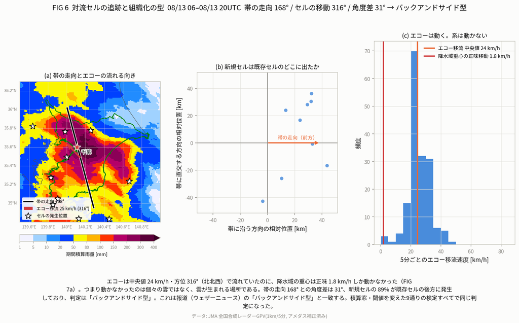
The angle difference slightly exceeds the classification boundary (30°) and fits the back-and-side-building definition (30–60°). New-cell locations are also rearward-dominant (89%) but with a substantial lateral share (44%), consistent with a “rear + side” description of the mode.
We checked three accumulation windows (full heavy-rain period, peak only, latter half only); all gave the same diagnosis.
This also matches media reports (Weathernews) of a “back-and-side-building” type.
https://weathernews.jp/news/202608/140101
On terrain
The term “linear precipitation band” has long entered public vocabulary, but the common image is strongly orographic: warm moist air keeps flowing into a mountain, rain clouds form and move, but successive formation at the same place makes the system appear fixed as a line.
Terrain influence has been suggested for this case as well, and that may play some role. Within the scope of this analysis, however, treating it as a convergence zone from cold-pool outflow opposing easterly warm moist flow fits the data better than terrain. Boso Peninsula topography is not steep enough to explain convergence of this scale on its own.
Determining whether terrain contributed would require checking whether past cases with similar synoptic setups repeatedly concentrate rain on the same axis. That remains future work.
2-5. Mechanism summary
Reorganized into four layers:
| Layer | Element | Figures / data checked |
|---|---|---|
| 1. Moisture supply | E–SE winds around the rim of a high east of the Kurils. Moisture from Typhoon 15 exited once and re-entered on the 13th (θe 328 → 348 K; precipitable water 41 → 60 mm) | FIG A |
| 2. Instability | Cut-off cold vortex. Trough axis upright from 1000–500 hPa (130–132°E); Chiba ~750 km east. 500 hPa −5.7 °C. Δθe 18–21 K before heavy rain | FIG B / FIG C / FIG D |
| 3. Forced ascent | Inland cold pool (Δθ −3.3 K) spreading east, opposed by easterlies (37 vs 28 km/h, same order). Observed front advance 5.1 km/h. But the model placed the convergence line 30–60 km southeast | FIG E / FIG 5c / FIG F |
| 4. Quasi-stationarity | Clouds kept flowing at 22–24 km/h (358 km in 14 h), but the band’s net motion was 25 km (1.8 km/h). Accumulation anisotropy 6.3× (AMeDAS 6.5×). Band width instantaneous 16 km / accumulated 40 km | FIG 6b / FIG 7 |
And the quantitative aspect matters. Even with the same structural setup, rain of this magnitude is not guaranteed. Moisture amount, mid-level cooling on the west side, and wind strength (gust front from the west; high-rim flow from the east)—these magnitudes can change the outcome by an order of magnitude. As Part 3 shows, what the model mainly missed appears to have been the wind side: the strength and location of convergence.
Part 3 — Predictability: what the model captured, and what it did not
3-0. What this part covers
Building on the mechanism in Part 2, we examine how far numerical weather prediction captured it—and, if not, which elements were missed.
Two caveats first.
First, what we examine here is the JMA MSM (Meso-Scale Model; ~5 km surface mesh). We have not treated the finer Local Forecast Model (LFM) in this article; reasons follow later.
Second, the attribution below depends heavily on back-calculation from residuals. We did not independently verify moisture amounts with observations; the discussion includes arguments of the form “even varying moisture cannot close the shortfall.”
3-1. When did rainfall become predictable?
Start with the simplest question: how well did MSM predict this rainfall?
Overall, this case is said to have been “hard to forecast.” That is fair—but looking inside the numbers yields a somewhat different picture.
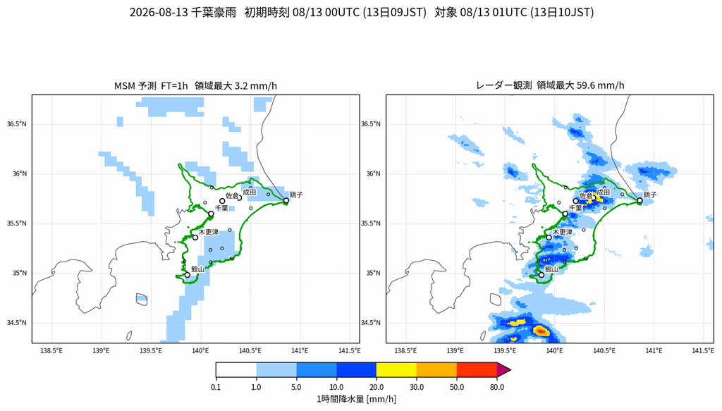
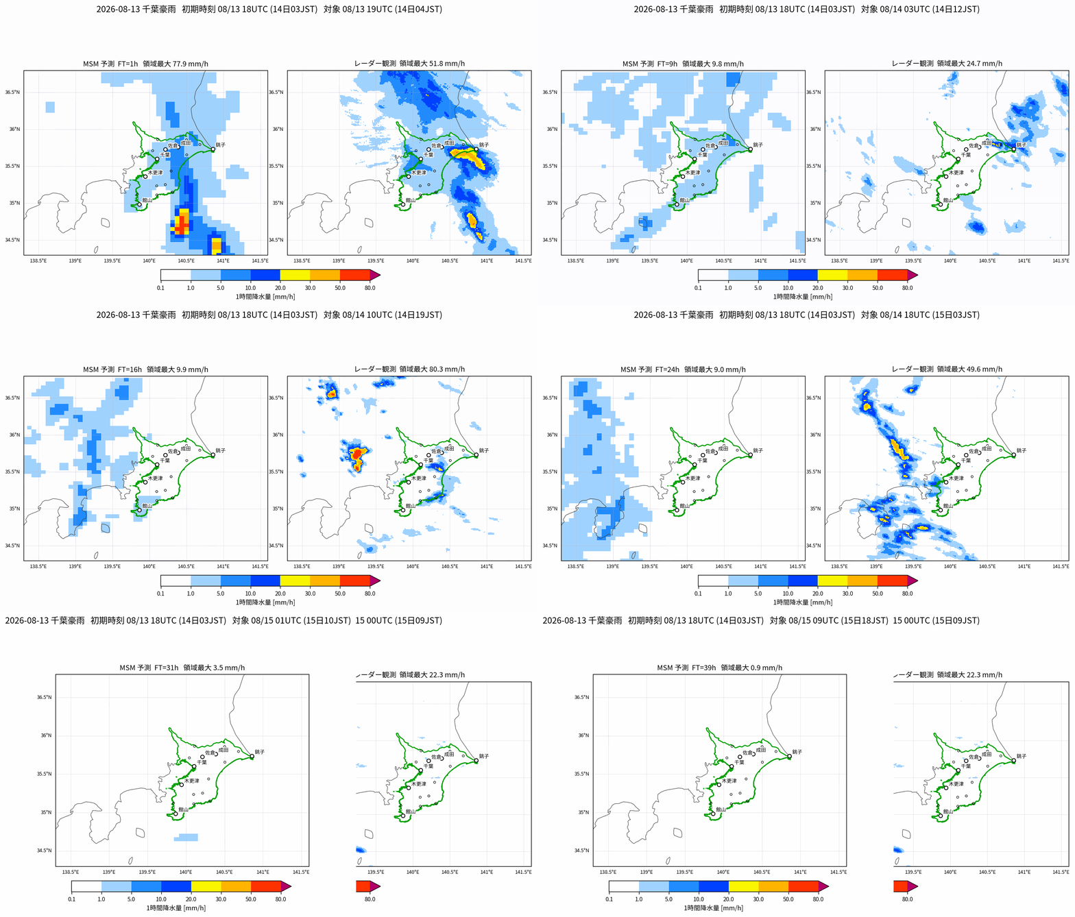
The animation above gives a rough comparison of MSM forecasts (initialized at 09 JST on the 13th) against radar-observed rainfall. MSM does forecast rain over Chiba, but it barely represents the intense rainfall that actually occurred.
Next we ask from when the rain in the critical 12 hours—8/13 09–21 JST (W1, including the 19:00 peak)—was predictable.
Reference figure: FIG 9. Forecast rainfall for the same valid time by initial time. Horizontal axis is lead time (older initials to the left).
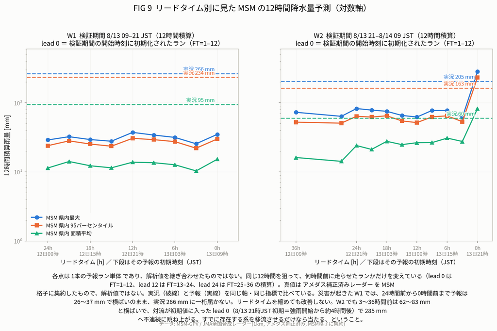
Left panel: maximum 12-hour precipitation within the prefecture for the critical 12 hours (8/13 09–21 JST), arranged by initial time (lead time).
| lead [h] | 24 | 21 | 18 | 15 | 12 | 9 | 6 | 3 | 0 |
|---|---|---|---|---|---|---|---|---|---|
| MSM [mm] | 29 | 32 | 29 | 28 | 37 | 34 | 32 | 26 | 35 |
At lead 0—i.e., the morning forecast at 09:00 on the day—forecast rainfall stayed in the 26–37 mm range, an order of magnitude short of the observed 266 mm. From 24 hours to 0 hours ahead, all nine runs sat in the same range; the forecast did not improve even on the morning of the day.
Next, for the following 12 hours—8/13 21 JST–8/14 09 JST (W2)—we ask from when the rain was predictable.
Right panel: maximum 12-hour precipitation within the prefecture for 8/13 21–8/14 09 JST, arranged by initial time (lead time).
Even at lead 3 hours—i.e., the 18:00 forecast—sufficiently intense rain was still not predicted. By then the first linear precipitation band (occurrence at 17:58) was already in place, and record short-term heavy rain information was being issued. Forecast rainfall nonetheless remained in the 62–83 mm range.
Only at lead 0—i.e., 21:00, roughly when the heavy-rain peak was being crossed—did the model become able to forecast the subsequent intense rain (285 mm).
In summary, the forecast only hit once the intense rain was already underway. Neither a few hours ahead, nor half a day ahead, could this magnitude of rain be spun up as a forecast.
Note: why we look at MSM
JMA also operates a finer Local Forecast Model (LFM). Since 17 March 2026, 1 km has been the standard horizontal resolution (the legacy 2 km version remains available as a transitional product, planned for end of service around March 2028). Forecasts from 00, 03, 06, 09, 12, 15, 18, and 21 UTC extend to 18 hours; forecasts from other hourly initials extend to 10 hours.
In resolution terms, LFM is clearly better suited to a ~16 km-wide convergence line. LFM may look quite different, and further analysis is needed.
We still focus on MSM here because our aim is forecasts days ahead. With forecast lengths of 10–18 hours, LFM structurally lacks the lead time needed for evacuation and pre-deployment decisions. If the question is whether one can prepare days ahead, we need to know what is and is not possible on MSM’s playing field.
3-2. Why intense rain appeared only from the 21:00 initial
As seen above, only from 21:00 on 8/13 (W2 lead 0) could the model forecast subsequent intense rain. Why was 21:00 the threshold?
With and without an existing system, the outcome is completely different
21:00 has a clear meaning. By then, the first intense rain (19:00 peak) had already occurred, and a convective system actually existed in the analysis. The forecast initialized at 21:00 did not invent new rain from a blank slate; it evolved a system that was already there.
That difference is clear in the evolution of convergence (the process that gathers moisture into one place). For the 21:00-initialized run, comparing the initial time (FT+0) with three hours later (FT+3, 00:00 on the 14th):
| FT | Valid time (JST) | Convergence in this run [mm/h] | Prefecture-mean forecast rain [mm/h] | Radar observation (mean) |
|---|---|---|---|---|
| 0 | 21:00 on the 13th | 4.69 | — | 8.08 |
| +3 | 00:00 on the 14th | 9.88 | 11.61 | 8.03 |
| +6 | 03:00 on the 14th | 0.45 | 6.34 | 5.97 |
Convergence did not decay; within three hours it grew to 2.1× the initial value. Rainfall was also reproduced to slightly above the observed mean.
Convergence may be better seen not as a “given amount,” but as an amount “produced by convection itself”
That makes sense given the nature of convergence. It is not a fixed quantity supplied from the initial condition; it is produced by a self-amplifying chain (feedback): cumulonimbus clouds condense water vapor and release heat → the air column warms and ascent strengthens → new low-level convergence forms → still more moisture gathers.
In other words, if a convective “seed” is already in the initial condition, the model can generate subsequent convergence on its own within a few hours.
Conversely, when the seed is not yet present (e.g., 09:00 initials for W1), the chain never starts. That is why forecast rainfall stayed capped at 26–37 mm whether 24 hours or immediately ahead.
The main locus of model bias in this case appears less to be the amount of water in the initial condition than the inability to spin up a convective system as a forecast before that system already exists in the analysis.
3-3. Source of the shortfall (1): moisture amount
So where does the shortfall come from? We examine the candidates in turn.
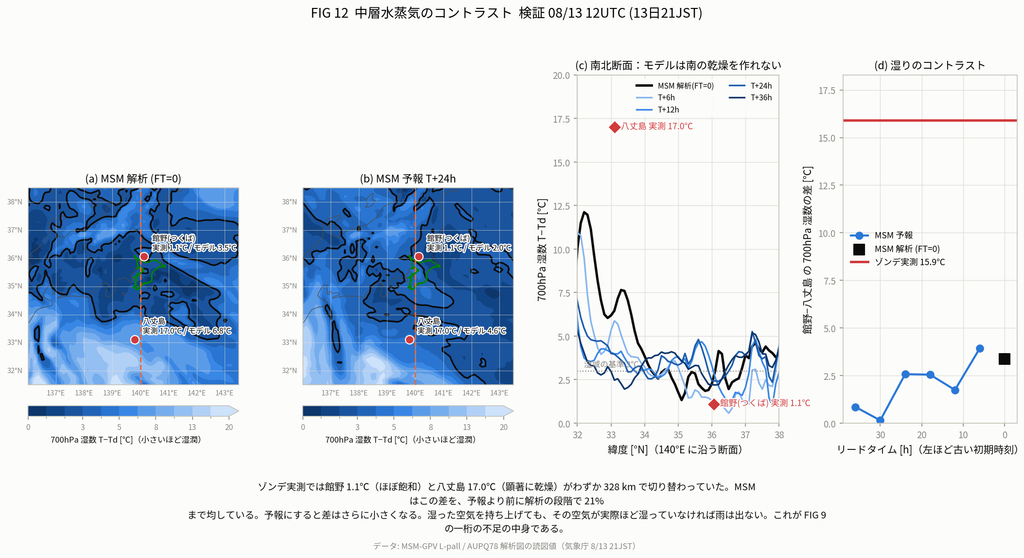
A natural first idea is that the model simply lacked enough water vapor. Indeed, as FIG 12 later shows, MSM substantially smooths the spatial contrast of mid-level moisture.
Looking at the amount itself, however, the picture is different. Precipitable water over Chiba (8/13 12 UTC) is as follows.
| Precipitable water [mm] | Ratio to analysis | |
|---|---|---|
| MSM analysis | 60.0 | 1.00 |
| Forecast lead 6 h | 58.0 | 0.97 |
| Forecast lead 24 h | 56.0 | 0.93 |
| Forecast lead 36 h | 55.2 | 0.92 |
Even a 36-hour forecast still held 92% of the analysis moisture. 60 mm itself well exceeds the heavy-rain rule of thumb of 50 mm. A fairly moist environment was already built inside the model.
What if we moistened it further? We computed the sensitivity.
| Condition | Precipitable water [mm] | Increase from analysis |
|---|---|---|
| MSM analysis (actual) | 60.0 | (baseline) |
| 700 hPa corrected to observed dewpoint depression 1.1 °C | 61.4 | +2.3% |
| 600–800 hPa set to dewpoint depression 1.1 °C | 61.9 | +3.1% |
| Full column set to dewpoint depression 1.1 °C (quite extreme) | 62.3 | +3.7% |
| Full column RH = 100% (physical upper bound) | 67.0 | +11.6% |
Even moistening the atmosphere to its physical upper bound increases precipitable water by only about 12%. Closing the shortfall seen in 3-2 would require roughly doubling the supply (+100%).
Therefore, correcting moisture amount may help fill part of the low bias, but is unlikely to explain the shortfall as a whole—that is our current view.
Caveat: this argument does not use an independent observation of precipitable water. We could not obtain GNSS-PWV or raw radiosonde data for this case; the moisture-bias discussion remains indirect, based on the physical-upper-bound argument above.
Moisture “distribution” was indeed smoothed
On distribution rather than amount, it is clear that the model did not fully capture reality.
Reference figure: FIG 12 — north–south contrast of 700 hPa dewpoint depression. Sonde observations versus MSM analysis and forecasts.
Specialized chart readouts (AUPQ78) show 700 hPa dewpoint depression of 1.1 °C at Tateno (Tsukuba; nearly saturated) and 17.0 °C at Hachijojima (markedly dry)—a 15.9 °C contrast over only 328 km. MSM analysis represents only 3.4 °C of that contrast—i.e., 21% of the observed difference. Forecasts shrink it further.
Whether this “smoothed distribution” is a direct cause of the rainfall shortfall is not something this analysis can show; for now it is better understood as a symptom of the model’s inability to resolve mesoscale boundary structure.
3-4. Source of the shortfall (2): strength of convergence
Next we look at the side that gathers moisture into one place—convergence. The question differs from the previous section. Section 3-2 asked how “this run,” once a convective seed was present at 21:00, evolved afterward. Here we ask: for convergence at one verification time—21:00 on the 13th—from how many hours ahead could it be forecast? Note that even for the same quantity, the axis of inquiry is reversed.
Vertically integrated moisture-flux convergence −∇·(qV) over Chiba Prefecture was decomposed into a mass-convergence term (−q∇·V; contribution from wind converging) and an advection term (−V·∇q; contribution from crossing a moisture gradient).
| Mass convergence −q∇·V | Advection −V·∇q | Total | Ratio to analysis | |
|---|---|---|---|---|
| MSM analysis | 4.82 | −0.13 | 4.69 | 1.00 |
| Forecast lead 6 h | 1.34 | −0.05 | 1.29 | 0.27 |
| Forecast lead 12 h | 1.07 | −0.34 | 0.73 | 0.16 |
| Forecast lead 24 h | 0.86 | −0.36 | 0.50 | 0.11 |
| Forecast lead 36 h | 0.39 | −0.47 | −0.08 | −0.02 (divergence) |
Units are mm/h. This table asks how far ahead the outcome at 21:00 on the 13th was predictable; as lead time lengthens (earlier initials), convergence falls to 8–28% of the analysis, and at 36 hours the sign finally reverses.
Almost all of what is missing is in the mass-convergence term—the side of wind converging. The advection term is only −0.13 mm/h even in the analysis; its quantitative contribution was limited.
That is consistent with the structure in Part 2. What produced this rain was a ~16 km-wide convergence line where a gust front opposed easterly warm moist flow. MSM pressure-level data are on an ~10 km mesh at 3-hour intervals. Representing a 16 km-wide structure on a 10 km mesh is principledly difficult (at least 4–6 grid cells, ~40–60 km, would be needed). Convergence values shown here should all be treated as lower bounds; the model’s internal state may have been stronger.
3-5. Source of the shortfall (3): location of the convergence band
Alongside strength, location error also mattered.
Reference figure: FIG F (FIGF_convergence_line.png, reprinted) — convergence line extracted from MSM surface winds.
As noted in Part 2, the MSM convergence-band centroid across six times lies at 34.9–35.6°N / 140.5–140.7°E—30–60 km southeast of Chiba City (35.60°N, 140.11°E). If the search domain is not limited to around Chiba Prefecture, the strongest surface convergence in MSM appears over the sea southeast of the Boso Peninsula.
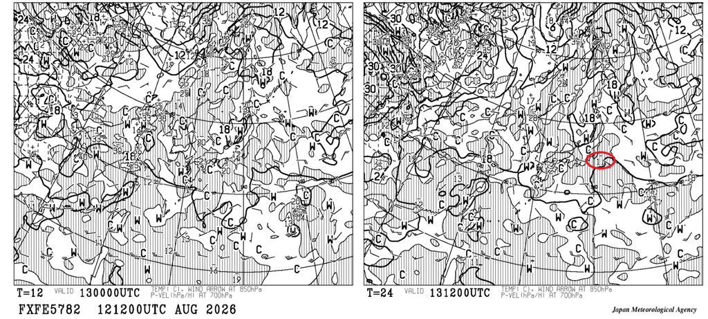
Personally, this point had bothered us since first looking at specialized charts. On the specialized chart (FXFE5782; initialized 21 JST on 8/12, 24-hour forecast valid 21 JST on 8/13), 700 hPa ascent was indeed forecast near Chiba. But the location was somewhat east–southeast, and the strength around −11 hPa/h felt weak for rain of this magnitude. Analyzing MSM confirmed that discomfort in the data.
When location shifts tens of kilometers southeast, the convergence line is placed over the sea rather than land. The precipitation maximum also goes offshore. Even if intensity were correct, it would not lead to urban (pluvial) flooding in central Chiba.
3-6. Organizing it as a three-layer structure
Putting this together, it cannot be written as a single simple chain (weak analysis → weaker forecast → location also wrong). Correctly, behavior is completely different depending on whether a convective seed is already present.
[Stage without a convective seed yet] (W1: 09:00 etc., up to 12 hours before the disaster)
Convergence cannot be spun up in the forecast
↓ Background: for a ~16 km-wide convergence line, L-pall is ~10 km mesh / 3-hourly and
cannot resolve it in principle
Forecast rainfall capped at 26–37 mm (observed 266 mm)
[Stage with a convective seed already present] (W2: 21:00 initial)
With a seed, convergence self-amplifies (2.1× analysis by FT+3)
↓
Rainfall can also be reproduced to near observed levels (though the simultaneous convergence-band location is still 30–60 km southeast)
Moisture amount, regardless of seed presence, was already ~92% of analysis even 36 hours ahead, and moistening to the physical upper bound adds only ~+12%. Our current understanding is: “The model largely had the water. What it could not do was gather it and spin up a convective ‘seed’ as a forecast before that seed already existed.” In addition, location error of the convergence band contributed to underestimating rainfall over Chiba.
Limits of this framing
As repeated above, this attribution has the following limits. Please read it with them in mind.
- No independent moisture observations. Neither GNSS-PWV nor raw sonde data were available. “The amount was adequate” is an indirect inference from the physical-upper-bound argument.
- Convergence shortfall is back-calculated from residuals. It was not measured directly.
- Convergence values are from L-pall and remain lower bounds given the resolution. The model’s native state (5 km mesh) may be finer.
- We look only at MSM. With different resolution, LFM may not support the same three-layer structure.
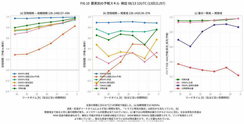
By element, forecast skill at synoptic scale (128–148°E / 27–43°N) keeps 500 hPa height and temperature correlations above 0.97 even at 36-hour lead—“approach of the upper trough and cold air” was reliably forecast from the previous day. Restricting to the Kanto domain (138–142°E / 34–37°N) lowers correlations for the same fields. The picture is: the large-scale pattern was right; mesoscale placement was wrong.
Reference figure: FIG 10 (FIG10_skill_by_element.png) — forecast skill by element and domain, synoptic scale versus Kanto domain side by side.
3-7. Where does it make sense to focus next?
Based on the above, we record our current thinking. This is not a definitive prescription, but work in progress.
As a premise, this analysis is MSM-based; comparison with LFM analysis is needed. For a ~16 km-wide convergence line, a 2 km mesh (or the 1 km product available since March 2026) should represent it better from a resolution standpoint.
As noted, however, LFM forecast length is 10–18 hours. For our goal of forecasts days ahead, LFM alone is not enough. “Solvable by LFM” and “preparable days ahead” are different problems; both need to be pursued.
Observations and assimilation
Technically, increasing observations and improving assimilation of them may raise performance.
Moisture observations (GNSS-PWV, etc.) were only partially helpful for closing a quantitative shortfall in this study. Capturing spatial moisture contrast may still help indirectly in resolving boundary structure.
In addition, wind observations look important. Doppler-radar radial winds, wind profilers, dense surface wind networks, and so on. As Section 3-2 showed, once a convective seed is in the analysis, convergence self-amplifies inside the model. The key is therefore capturing low-level wind convergence—the trigger of convection itself, such as gust fronts and easterly pushback—before a seed exists. How far observations can capture that “first push” before latent-heat feedback takes over likely governs whether convection can be spun up as a forecast.
From materials of the Working Group on Improving Linear Precipitation Band Forecast Accuracy, the top challenge has been seen as capturing moisture inflow—especially over the sea. This case additionally underscores the importance of wind observations.
Stronger assimilation is needed in parallel with model improvement, from the standpoint of how accurately the seed itself can be brought into the initial condition.
Room for AI contribution
People sometimes say “AI will solve everything” or “AI can forecast perfectly.” We do not think that is right.
Much of today’s weather AI trains on physical-model simulation output—i.e., reanalysis. For this case that is suggestive: even at reanalysis (analysis, t=0)—before forecasting—location and strength of the convergence band already showed errors. An AI trained on that data as teacher is hard to imagine suddenly forecasting the same case accurately. The principle that AI cannot exceed the quality of its training data applies here.
On the other hand, with hindsight, data for intense rain of this kind do exist, and understanding of the mechanism has advanced to some degree. If independent observations such as radar and AMeDAS are used as teacher data instead of reanalysis, and if architectures and inputs are designed around mechanisms revealed here (a convergence line tens of kilometers wide, and what forms it), we believe AI can still contribute meaningfully to forecast skill.
What can be done in operations today
We continually ask whether there is a last-mile contribution—built on JMA models—for events like this that the models alone do not reach. The Level 5 heavy rain special warning was issued at 19:30; if specialized insight could have caught danger signs earlier, two points stand out.
Simultaneous sharp changes in AMeDAS wind direction, temperature, and pressure At Chiba AMeDAS at 18:10 JST, a sharp wind shift (NNE→NW), wind-speed increase (7.9 m/s), temperature drop, pressure rise, and surge in 10-minute rainfall occurred together. That is passage of the convergence line itself. It reports boundary location earlier than radar, and far earlier than NWP.
Catch the latest forecast–observation divergence This is something we actually do: specialized forecast charts based on model NWP are issued twice daily (9am/9pm), but fresher insight often comes from the latest radar, AMeDAS, and satellite imagery. In this case, forecasts of 26–37 mm (12-hour rainfall) sat against observed 1-hour rates exceeding 100 mm/h. At that point, bias in the wind field and other assumptions of the model could have been detected and used to inform subsequent forecasts.
3-8. Closing
What we believe this analysis supports so far is the following.
- MSM underforecast this rainfall by a factor of about 7–10 regardless of lead time
- This was not only a forecast problem; similar underestimation appeared even in analysis rainfall at the 8/13 18:00 initial (t=0), as the rainfall peak was being approached
- On the other hand, once a convective seed was already in the analysis (from 21:00 onward), the model self-amplified convergence and reproduced intensity fairly well
- Moisture amount appears to have been present to a reasonable degree inside the model
- The main shortfall likely lay in the strength of convergence that gathers moisture into one place (and the generation of a convective seed that goes with it), and in its location
- In the background is a resolution limit relative to a ~16 km-wide convergence line
All of this remains preliminary analysis; parts still lack independent observational corroboration.
Going forward, we want to revisit the same case with higher-resolution models such as LFM, and to examine how far AI changes what when applied in practice. We will share progress as it comes.
If you are interested in our solution, please do not hesitate to reach out to us.